Refits the Kernel ODE model using a pre-specified regulatory network, bypassing the network estimation step.
Usage
refit_kernel_ODE(
  Y,
  obs_time,
  yy_smth,
  tt,
  kernel,
  kernel_params,
  interaction_term,
  adj_matrix,
  theta_initial = NULL,
  nzero_thres = NULL,
  tol = 0.001,
  max_iter = 10,
  verbose = 0
)
Arguments
- Y
A numeric matrix of dimension (
n,p), where each column corresponds to the observed trajectory of a variable. Rows align withobs_time.- obs_time
A numeric vector of length
nrepresenting observation time points.- yy_smth
A numeric matrix of dimension (
length(tt),p), where each column contains the smoothed trajectory of a variable evaluated ontt. This is typically the output ofkernelODE_step1().- tt
A numeric vector representing a finer time grid used for evaluating the smoothed trajectories and their derivatives.
- kernel
Kernel function to use.
- kernel_params
A list of length
p, where each element is a named list of parameters for a specific variable (e.g.,list(bandwidth = 1)for Gaussian kernel). If the list has length 1, the same parameter set is used for all variables. This is typically the output ofauto_select_kernel_params().- interaction_term
A logical value specifying whether to include interaction effects in the model.
- adj_matrix
An adjacency matrix (
p×p) representing the regulatory network to use for refitting. Entry(k, j) = 1indicates variablekregulates variablej. Typically obtained from a previous Kernel ODE estimation. IfNULL, defaults to a fully connected network. Although technically possible, this function is not intended for estimating \(F_j\) or inferring a regulatory network.- theta_initial
A numeric matrix containing the initial \(\theta_j\) values for each variable at the start of optimization:
If
interaction_term = FALSE,theta_initialmust have dimensions (p,p).If
interaction_term = TRUE,theta_initialmust have dimensions (p^2,p). IfNULL, defaults to all ones.
- nzero_thres
A number in
[0, 1]specifying the maximum proportion of nonzero regulators (edges) allowed for each variable (i.e., at mostp * nzero_thresregulators). Only used whenadj_matrixisNULL. This provides a faster alternative to the computationally expensive pruning process.- tol
Convergence tolerance for the relative improvement in the Frobenius norm of the \(\theta\) matrix.
- max_iter
Maximum number of iterations for the optimization.
- verbose
Integer; if greater than 0, prints progress messages during optimization.
Value
A list with components:
metricsRecovery metrics for the trajectories under the given network, including the overall \(R^2\) and variable-specific \(R^2\) values. See
assess_recov_traj().Y_refitRecovered trajectories from the refitted model, in the same format as
Y.
Examples
set.seed(1)
obs_time <- seq(0, 1, length.out = 10)
Y <- cbind(sin(2 * pi * obs_time), cos(4 * pi * obs_time)) + 0.1 * matrix(rnorm(20), 10, 2) # each col is a variable
tt <- seq(0, 1, length.out = 100)
res_step1 <- kernelODE_step1(Y = Y, obs_time = obs_time, tt = tt)
kernel <- "gaussian"
kernel_params <- auto_select_kernel_params(kernel = kernel, Y = Y)
res_step2 <- kernelODE_step2(Y = Y, obs_time = obs_time, yy_smth = res_step1$yy_smth, tt = tt, kernel = kernel, kernel_params = kernel_params)
network_est <- res_step2$network_est
# refit Kernel ODE using the estimated network
res_refit <- refit_kernel_ODE(Y = Y,
obs_time = obs_time,
yy_smth = res_step1$yy_smth,
tt = tt,
kernel = kernel,
kernel_params = kernel_params,
interaction_term = F,
adj_matrix = network_est) # the estimated network
(metrics <- res_refit$metrics)
#> $R2
#> [1] 0.4514784
#>
#> $R2_per_var_vec
#> [1] 0.9029567 0.0000000
#>
Y_refit <- res_refit$Y_refit
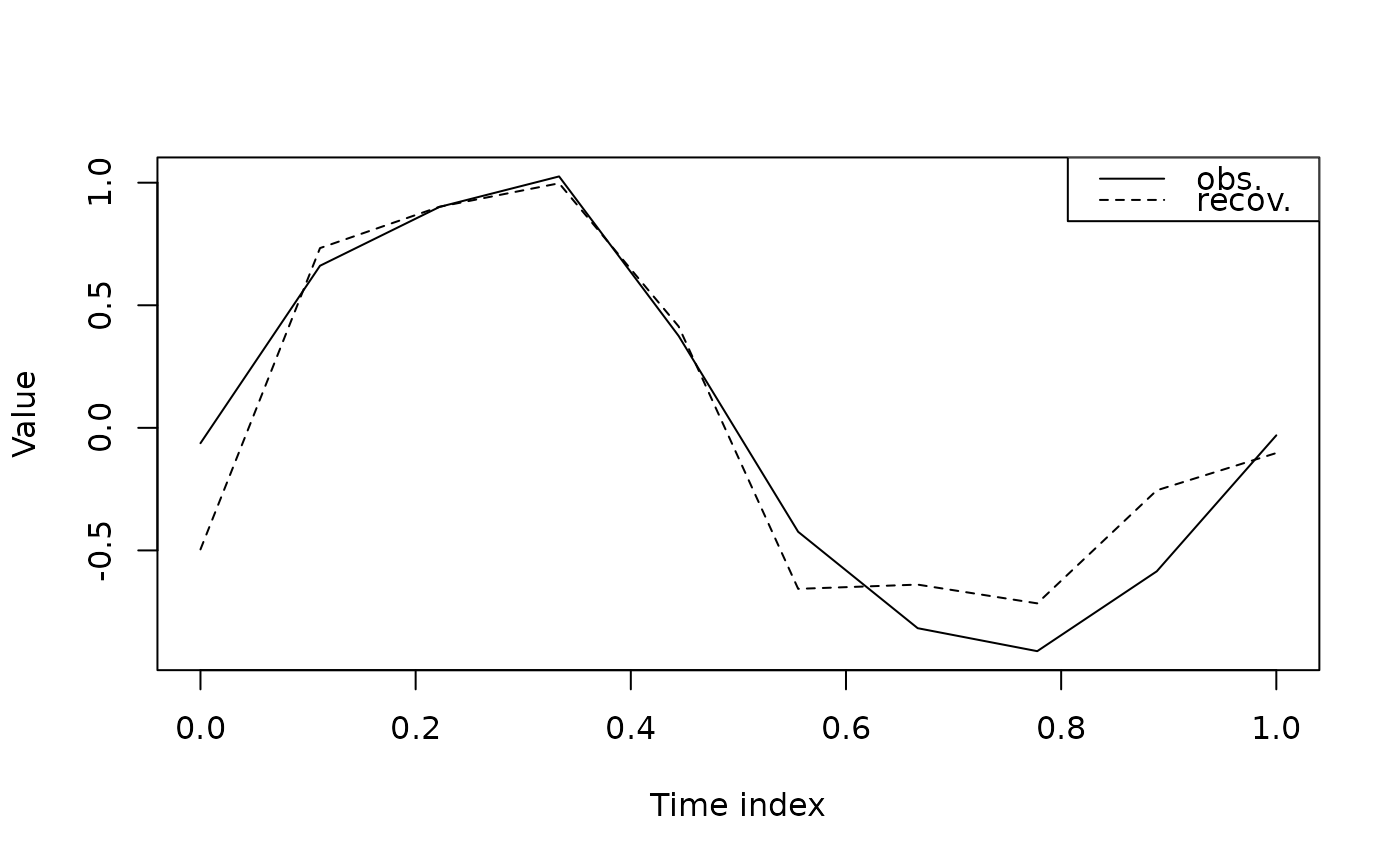
# plot the recovered traj
j <- 1
plot(NA, type = "n",
xlab = "Time index", ylab = "Value",
xlim = c(0,1), ylim = range(c(Y_refit[,j], Y[,j]), na.rm = T))
lines(obs_time, Y[,j], lty = 1)
lines(obs_time, Y_refit[,j], lty = 2)
legend("topright",
legend = c("obs.", "recov."),
lty = c(1,2),
col = "black")