Smoothing Spline Estimates (Step 1 of Kernel ODE)

Computes smoothed trajectories and their derivatives using cubic smoothing splines. This function serves as Step 1 in the Kernel ODE pipeline.

Usage

kernelODE_step1(Y, obs_time, tt)

Arguments

Y

A numeric matrix of dimension (n, p), where each column corresponds to the observed trajectory of a variable. Rows align with obs_time.

obs_time

A numeric vector of length n representing observation time points.

tt

A numeric vector representing a finer time grid used for evaluating the smoothed trajectories and their derivatives.

Value

A list with components:

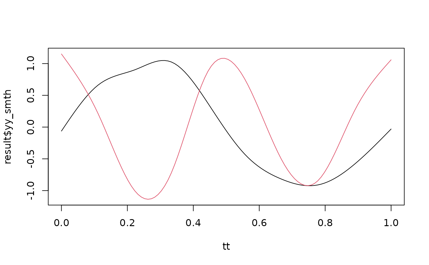
yy_smth

A numeric matrix of dimension (length(tt), p), where each column contains the smoothed trajectory of a variable evaluated on tt.

init_vals_smth

A numeric vector of length p containing the estimated initial values (at time 0) for each variable.

deriv_smth

A numeric matrix of dimension (length(tt), p), where each column contains the smoothed first order derivative of a variable evaluated on tt.

References

Original implementation adapted from https://github.com/ChenShizhe/GRADE

Examples

# Example usage:
set.seed(1)
obs_time <- seq(0, 1, length.out = 10)
Y <- cbind(sin(2 * pi * obs_time), cos(4 * pi * obs_time)) + 0.1 * matrix(rnorm(20), 10, 2)  # each col is a variable
tt <- seq(0, 1, length.out = 100)
result <- kernelODE_step1(Y = Y, obs_time = obs_time, tt = tt)
matplot(tt, result$yy_smth, type = "l", lty = 1, col = 1:2)